A pseudorandom number generator produces numbers deterministically but they seem aperiodic (random) most of the time for most use-cases. The generator accepts a seed value (ideally a true random number) and starts producing the sequence as a function of this seed and/or a previous number of the sequence. These are Pseudorandom (not truly random) because if seed value is known they can be determined algorithmically. True random numbers are hardware generated or generated from blood volume pulse, atmospheric pressure, thermal noise, quantum phenomenon, etc.
There are lots of techniques to generate Pseudorandom numbers, namely: Blum Blum Shub algorithm, Middle-square method, Lagged Fibonacci generator, etc. Today we dive deep into Rule 30 that uses a controversial science called Cellular Automaton. This method passes many standard tests for randomness and was used in Mathematica for generating random integers.
Cellular Automaton
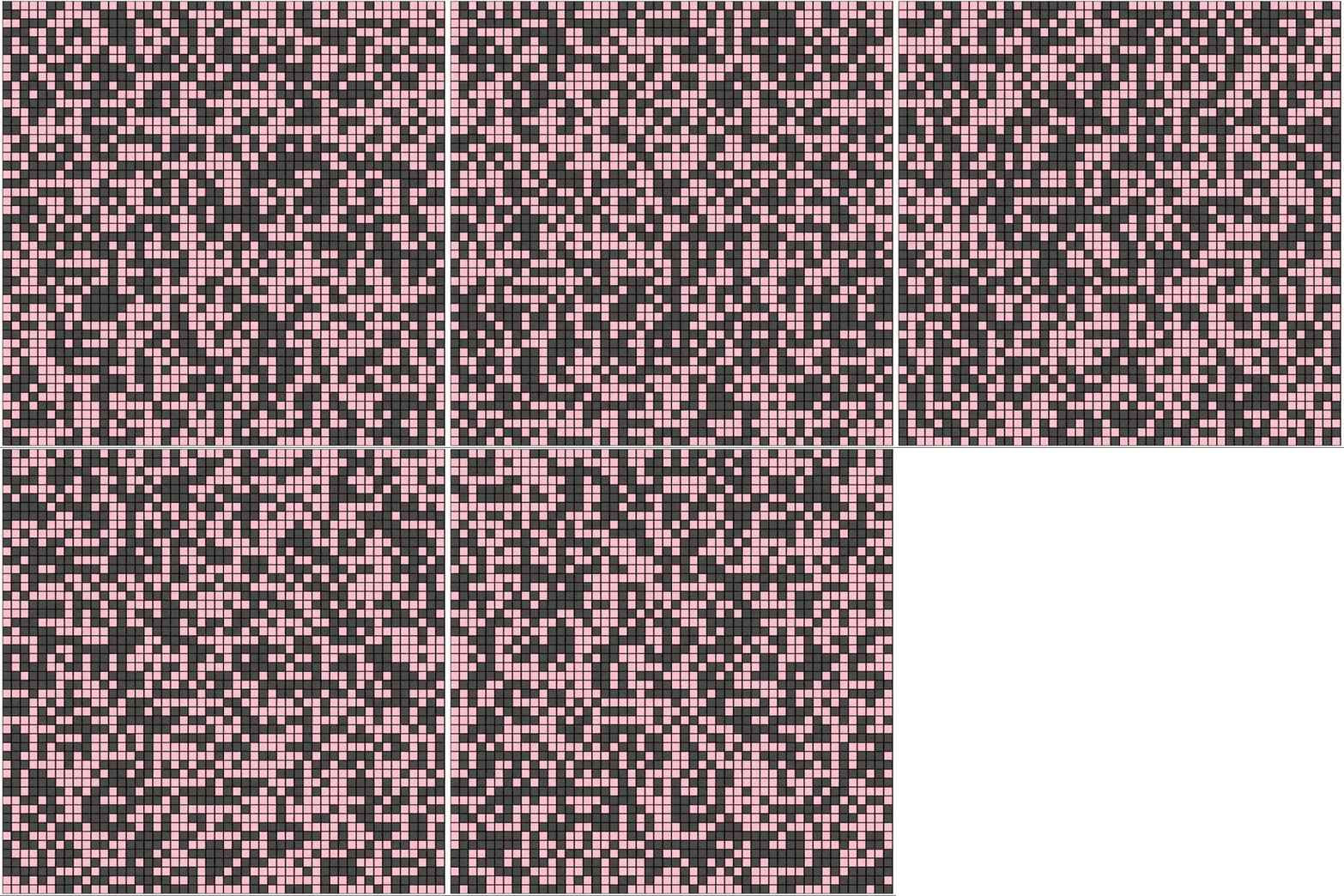
Before we dive into Rule 30, we will spend some time understanding Cellular Automaton. A Cellular Automaton is a discrete model consisting of a regular grid, of any dimension, with each cell of the grid having a finite number of states and a neighborhood definition. There are rules that determine how these cells interact and transition into the next generation (state). The rules are mostly mathematical/programmable functions that depend on the current state of the cell and its neighborhood.

In the above Cellular Automaton, each cell has 2 finite states 0 (shown in red), 1 (shown in black). Each cell transitions into the next generation by XORing the state values of its 8 neighbors. The first generation (initial state) of the grid is allocated at random and the state transitions, of the entire grid, is as below

Cellular Automata was originally conceptualized in the 1940s by Stanislaw Ulam and John von Neumann; it finds its application in computer science, mathematics, physics, complexity science, theoretical biology and microstructure modeling. In the 1980s, Stephen Wolfram did a systematic study of one-dimensional cellular automata (also called elementary cellular automata) on which Rule 30 is based.
Rule 30
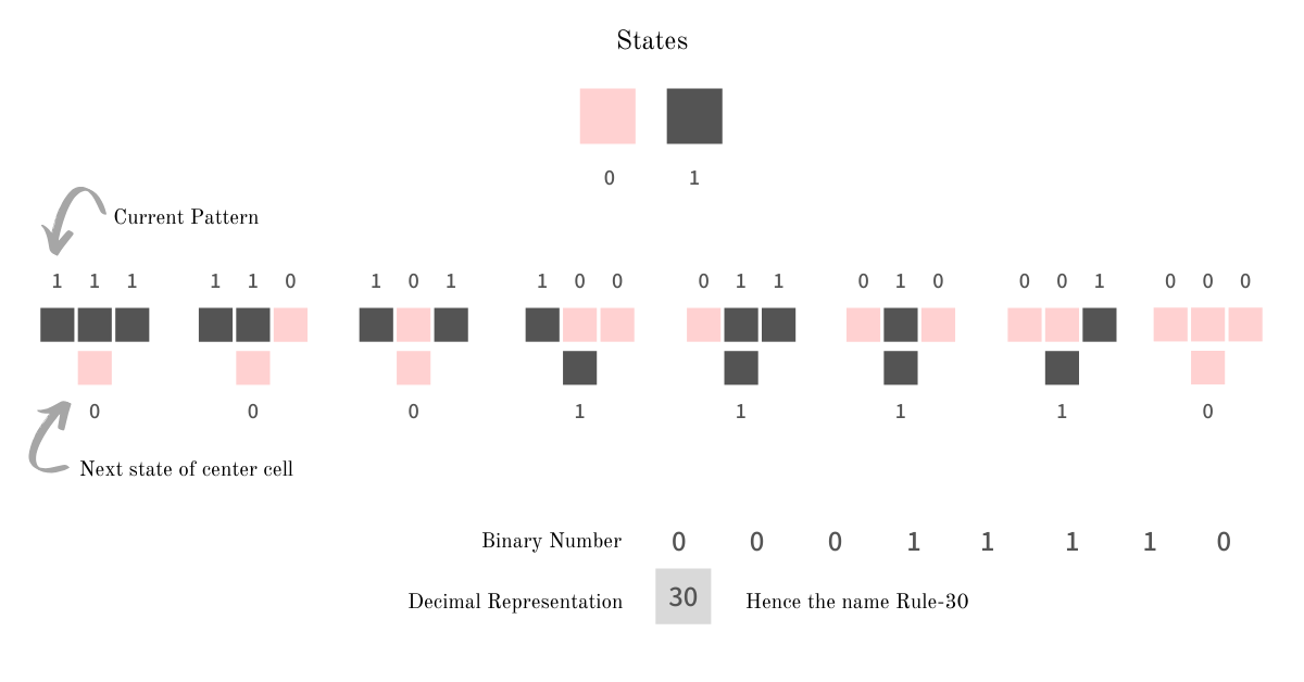
Rule 30 is an elementary (one-dimensional) cellular automaton where each cell has two possible states 0 (shown in red) and 1 (shown in black). The neighborhood of a cell is its two immediate neighbors, one on its left and other on right. The next state (generation) of the cell depends on its current state and the state of its neighbors; the transition rules are as illustrated below

The above transition rules could be simplified as left XOR (central OR right).
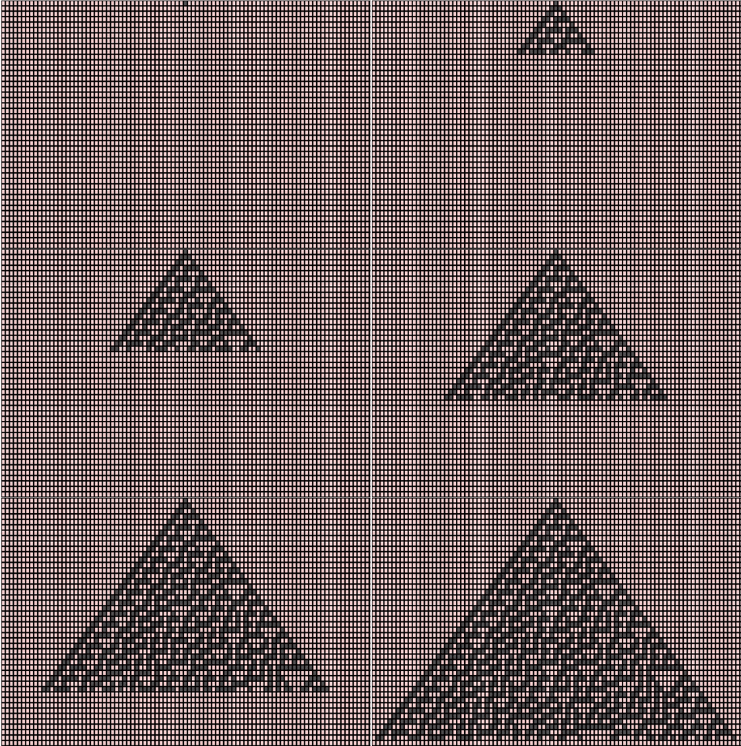
We visualize Rule 30 in a 2-dimensional grid where each row represents one generation (state). The next generation (state) of the cells is computed and populated in the row below. Each row contains a finite number of cells which “wraps around” at the end.

The above pattern emerges from an initial state (row 0) in a single cell with state 1 (shown as black) surrounded by cells with state 0 (red). The next generation (as seen in row 1) is computed using the rule chart mentioned above. The vertical axis represents time and any horizontal cross-section of the image represents the state of all the cells in the array at a specific point in the pattern’s evolution.

As the pattern evolves, frequent red triangles of varying sizes pop up but the structure as a whole has no recognizable pattern. The above snapshot of the grid was taken at a random point of time and we could observe chaos and aperiodicity. This property is exploited to generate pseudorandom numbers.
Pseudorandom Number Generation
As established earlier, Rule 30 is exhibits aperiodic and chaotic behavior and hence it produces complex, seemingly random patterns from simple, well-defined rules. To generate random numbers from using Rule 30 we use the center column and pick a batch of n random bits and form the required n bit random number from it. The next random number is built using the next n bits from the column.

If we always start from the first row, the sequence of the numbers we generate will always be predictable - which is not what we want. To make things pseudorandom, we take a random seed value (ex: current timestamp) and skip that number of bits and then pick batches of n and build random numbers.
The pseudorandom numbers generated using Rule 30 are not cryptographically secure but are suitable for simulation as long as we do not use bad seed like
0.
One major advantage of using Rule 30 to generate pseudorandom numbers is that we could generate multiple random numbers in parallel by picking multiple columns to batch n bits each at random. A sample 8-bit random integer sequence generated using this method with seed 0 is 220, 197, 147, 174, 117, 97, 149, 171, 240, 241, etc.
The seed value could also be used as the initial state (row 0) for Rule 30 and random numbers are then simply the n bits batches picked from the center column starting from row 0. This approach is more efficient but is heavily dependent on the quality of seed value, as a bad seed value could make things extremely predictable. A demonstration of this approach could be found on Wolfram Cloud Demonstration Page.
Rule 30 in the real world
Rule 30 is also seen in nature, on the shell of code snail species Conus textile. The Cambridge North railway station is decorated with architectural panels displaying the evolution of Rule 30.
Conclusion
If you found Rule 30 interesting I urge you to write your own simulation of using p5 library; you could keep it generic enough to so that the program could generate patterns for different rules like 90, 110, 117, etc. The patterns generated using these rules are quite interesting. If you want, you could things to the next level and extend rule to work in 3 dimensions and see how patterns evolve. I believe programming is fun when it is visual.
It is exciting when two seemingly unrelated fields, Cellular Automata and Cryptography, come together and create something wonderful. Although this algorithm is not widely used anymore, because of more efficient algorithms, it urges us to be creative in using Cellular Automata in more ways than one. This article is first in the series of Cellular Automata, so stay tuned and watch this space for more.
